Learn SQL Basics

SQL aka structured query language is the base for Pizza (Analytics and Data Science). While everyone goes gung-ho about the toppings and cheese (machine learning & fancy algorithms). SQL is critical for being able to query structured data for clear insights and start the analysis with the right questions. Thus the a need to learn SQL basics and beyond.

“Give me six hours to chop down a tree and I will spend the first four sharpening the axe.”

– Abraham Lincoln

Who is this for?

These notes/pointers are for folks (executives, new analysts etc) who are looking to set up or learn SQL basics to be able to do basic analytics from time to time. Anyone, who’s already worked extensively with data and does so regularly, can skip this.

Why is SQL necessary? I’m planning to do AI/ML

The analytics setup at any firm starts with 3 steps: Analytical Base + Data Engineering (Cheese) Middle Layer + Final Toppings of Data Science to customise and specialise the Pizza. Go through this write-up to understand how to set up an analytics program from scratch. To be able to set up the base correctly, one needs nothing more than a good DB setup and good old SQL. Learn SQL!

SQL Basics

The first setup of requirements for learning SQL is to be able to practice it thoroughly on a test workbench. Where one can quickly iterate over queries while learning basic commands etc. This may not necessarily be true for an internal database setup in the early days, where one might not have a proper engine setup correctly. The data might not be correct and we have no feedback loop on what’s a correct outcome. LearnSQL comes in handy here!

Querying from a Single Table

The simplest of the requirements will be around querying from a single table. We might be required to fetch only a subset of data. The commands help filter or choose a subset of rows or columns once the base data has been decided.

• SELECT *: Choose all columns present in the underlying table
• FROM: To choose the table of choice
• WHERE: Helps filter rows based on conditions.
  • >, <, =, != : Greater and Less than. Equal to and not equal to conditions. Goes with WHERE
  • BETWEEN: When choosing between a range of values. You can do the opposite by also using NOT BETWEEN.

• OR/AND: Operands to combine multiple conditions, possibly over multiple columns with different constraints.
• (Parenthesis) : Useful, when adding complex and long conditions, that are a mix of OR & ANDs.

• LIKE: This command is similar to ‘=’ but very useful when trying to do a partial match over strings.
  • % (Percent): The percentage sign is useful for a partial match like trying to match strings starting with a particular letter or sequence of letters and so on.
  • One caveat, SQL is case-sensitive when matching strings. ‘FORD’ is not the same as ‘Ford’.
  • SQL commands and syntax are not case-sensitive. Thus WHERE and where are both treated equally by the SQL engine.

• NULL: This keyword is used when one of the column values is missing. It’s a special case and is checked by using IS NULL or de-selected using IS NOT NULL. Equal to (=) does not work with NULL.
• Arithmetic: We can do basic arithmetic operations like multiply, divide, add and subtract numbers.

Multiple Tables

Now the goal is to take this further, by being able to query and fetch data from multiple tables. The same set of commands is useful but we will need to go beyond those by learning JOINs and beyond.

• SELECT *: When wanting to select columns from more than 1 table, we can choose SELECT * FROM table1, table2.
  • The output here is basically a combination of all rows in both thus the output being all rows in table1 X all rows in table2.

• JOIN/ON: This command combination is thereby useful to know how to combine two tables, JOIN tells the two tables and ON, how it’s to be done.
  • e.g. SELECT * FROM table1
  • JOIN table2 ON table1.id = table2.id

• SELECT Specific columns: When choosing specific columns from multiple tables, we can do so using SELECT table1.name, table2.name FROM table1 JOIN table2 ON and so on … We write the table names before the column names to exactly specify which columns from which tables.
  • The writing of the table names as prefixes is optional when the column names are unique and different between the tables.
  • But mentioning them explicitly irrespective is a good practice.

• AS: This is used as an alias for the column names. Only changes the name when being shown, the underlying table name still remains intact.

GROUP BY, STATISTICS and beyond

Besides being able to query and fetch data from multiple tables and filtering rows based on conditions, the next step is to be able to do summary stats. This requires a couple of commands like GROUP BY and so on.

• ORDER BY: This specific command is all about ordering the output from an SQL query basis a certain condition including values in a specific column and so on.
  • e.g. SELECT * FROM table1 ORDER BY table1.columnx
  • It’s the same set of data but the rows are now ordered by the values in the columns

Statistical Commands

• DISTINCT: Useful when selecting or looking for unique entries or unique combinations of occurrences instead of all.
• COUNT: Helps count rows in the specific output. Know the count of instances meeting our specific conditions.
• MAX/MIN: Max and Min help choose the maximum or the minimum values from a column in our tables.
• AVG: Average is one way to compute the average of the values from a specific column.

• GROUP_BY: This is the boss command besides where that will be used very frequently. It’s useful when aggregating certain columns subject to values in a specific column.
  • e.g. SELECT column1, COUNT(column2) FROM table1 GROUP BY column1
  • We are selecting column1 and the count of rows by using column1 in the group by. It tells how many times, column 1 occurs in the table.
  • In terms of the order of choosing GROUP BY and WHERE. We first filter rows of interest using WHERE and then Group them using GROUP BY.

HAVING Command

• HAVING: This is the command used along with GROUP BY and comes after the GROUP BY to be able to filter for specific rows basis the aggregate function on that column.
  • SELECT column1, COUNT(column2) FROM table1 GROUP BY column1 HAVING COUNT(column2) > 2
  • The same query but this time filtering for rows where the count is greater than 2

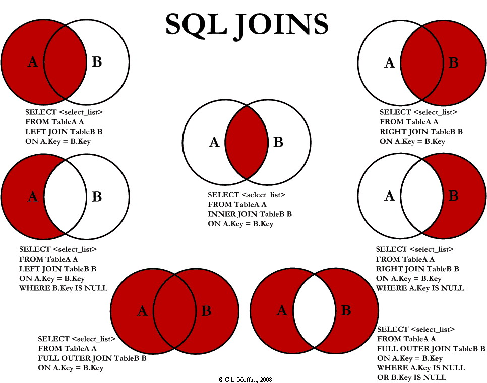
JOINs in Detail

There are broadly four joins in total, JOIN aka LEFT JOIN, INNER JOIN, RIGHT JOIN and CROSS JOIN. The differentiation is best visualised using the Venn diagram with the syntax being the same as above with change in the key words.

Subqueries

Subqueries are useful when we need to run a query within a query to be able to fetch the desired results. It’s kinda similar to the recursive functions in programming. Calling a function or query within another. There are often multiple ways to execute something through a sub-query vs a JOIN.

• Subquery: Typically is placed within rounded parentheses. You can filter rows or run complex queries where one of the conditions is the basis output from one of the subqueries.
  • e.g. Filter for all values from Table1 for some values less than a threshold in Table2.
  • We could do a LEFT JOIN and then explicitly filter for values in Table1 or we run a subquery within.

• Correlated Subquery: Subqueries can also depend on values from the main query. Thus correlated or dependent subqueries.
• ANY/ALL : These are some of operators useful when carrying out subqueries. Useful to compare when conditions from the main query compared against the output from the internal query.
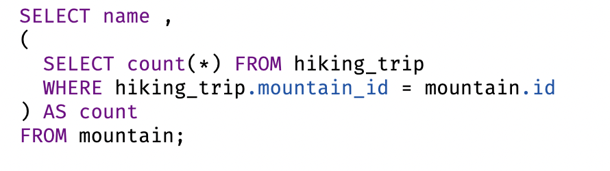
• AS : Sometimes, we might want to run a bunch of subqueries and save their outputs in form of temporary tables. We can give them names aka alias using the AS keyword.
  • We created a new column using a subquery and name it count
  • The main query was fetching names from the mountain.
  • The subquery fetched the column count.

UNION/INTERSECT

Besides these, there are a few basic set of commands to be able to combine outputs from multiple queries based on the set theory, namely UNION, INTERSECT.

• UNION: This combines the output from multiple queries. Like if you are fetching IDs from two queries and want an OR condition or a UNION, this command can help us combine the output and remove duplicates.
• INTERSECT: This is a representation of the AND condition, when the outputs occur in both queries, we will have the outputs.
• EXCEPT/MINUS: This is basically output from one query subtracted from another.

Why buy a paid course? SQL is available freely

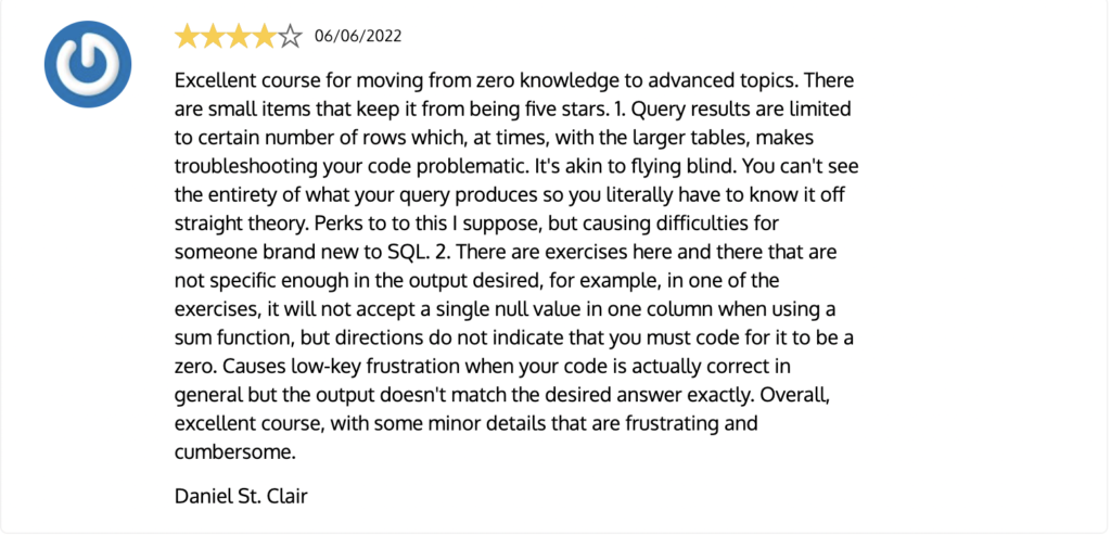
So, this wraps up all basic commands and their intent/usage patterns. The fastest way to pick these up is to go ahead and learn SQL basics from this course. It’s paid thus the platform works smoothly, you can practice different commands mentioned with a beautiful UI/UX. The money goes a long way in ensuring, you focus on learning. This course can be done dedicatedly in 2-3 days and goes a long way in making you self reliant.

email: admin@startupanalytics.in for any queries and questions.